Page History

...

• Analysis starts with the implementation of the Elliptical-Weighted-Average (EWA) algorithm within the PyResample open source Python implementation (with some Cython modules for speed)
• The PyResample implementation is based upon the implementation within the MODIS-Swath-to-Grid-Toolbox(MS2GT) developed and distributed by NSIDC.  See: https://nsidc.org/data/user-resources/help-center/what-modis-swath-grid-toolbox-ms2gt-and-what-can-it-do
• MS2GT is based upon an algorithm developed by Green & Heckbert, IEEE, June 1986
  "Creating Raster Omnimax Images from Multiple Perspective Views Using the Elliptical Weighted Average Filter".
  https://ieeexplore.ieee.org/document/4056910
• None of this provides much clarity in defining the image characteristics and performance of the algorithm.
• See also, as an introduction two wiki pages I developed a few years back: ESDIS-SDPS Earth-Data Projection Introduction and Forward-Projection and Reverse-Projection Algorithms

The EWA Algorithm for swath data projection is a highly efficient and well-established approach for projecting Earth-Observational swath data to a “regular grid”.  It likely also has some possible “off-label” applications to projecting geographically gridded data and general data regridding - without reprojection (shifting grid alignment and changing resolution), and possibly also . Another possible application would be to general reprojection of projected grids.

...

• EWA was developed at NSIDC for MODIS swath data handling, circa 1990’s. Originally developed (and still available) as part of MODIS Swath-to-Grid Toolbox (MS2GT)
• It is designed and capable of handling swath data with multiple rows of data containing data points “across-track” per scan (rows being “along-track”). Such data can exhibit the so-called “bow-tie” effect where the sample-spot (data cell) reflects an increasing area away from the nadir observation directly below the satellite.  This includes side to side angular stretching, as well as some forwards and backwards stretching across multiple scan-rows of data.  These angular perspectives create an elliptical stretch of the sample-spot away from the center of the scan.

• Expand
  title More details...
  The original IEEE article shows a diagram showing the elliptical source cell to target cell mapping (shown left to right below).  This corresponds to the stretching of the data acquisition sample spot when off nadir , from the satellite instrument instrument.

Comparison of swath projection and grid reprojection

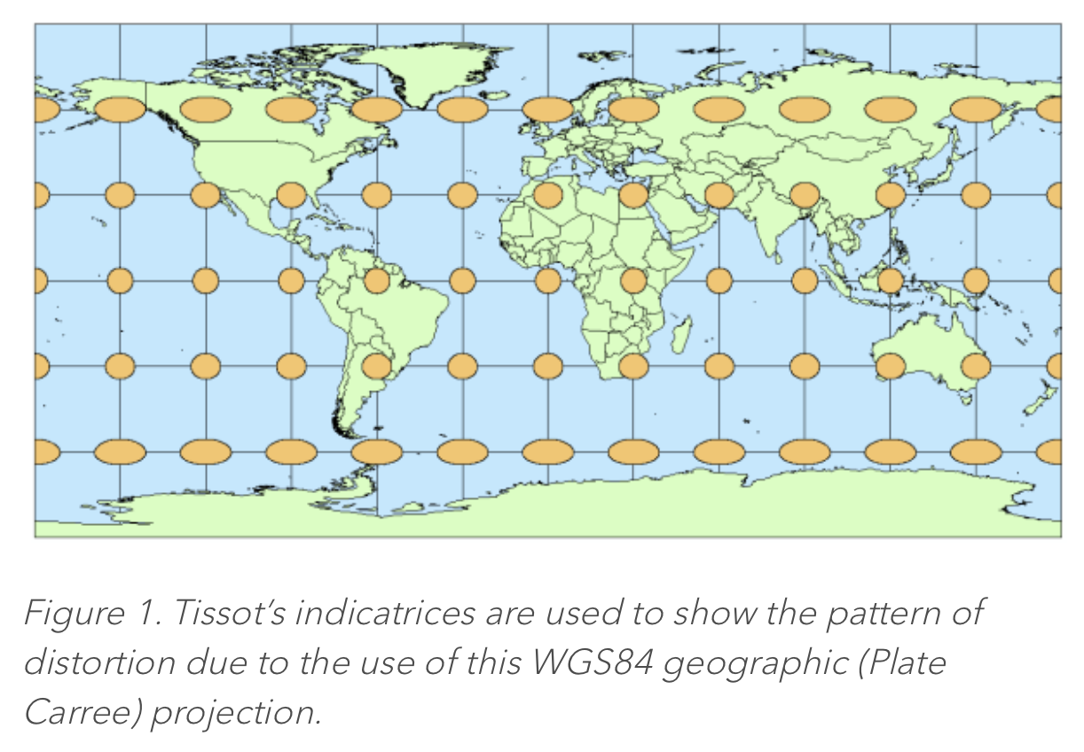
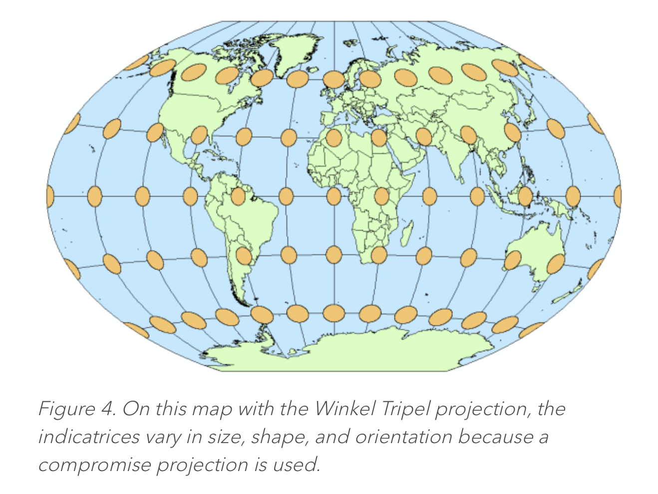
• Note that the elliptical perspective of the EWA algorithm for swath data is quite similar to the Tissot Indicatrix ellipse of earth-data-to-flat-map projections – which shows the east-west and north-south angular distortion of a projection. More There will be more discussion on this later in “off-label” applications of the EWA algorithm.  [Application of EWA for grids would not involve multiple rows-per-scan of swath data acquisition, rather referring to just one row of projected data per step along track (rows-per-scan = 1)].
• In fact, even within the EWA algorithm, there is the elliptical area of the "sample-spot", and there is a Tissot ellipse of projection stretch (distortion) of the sample spot to a flat-earth grid.  The algorithm does not particularly focus on these two sources of elliptical coverage separately, but simply computes an ellipse of coverage from the source data to the target grid.

• Expand
  title More details...
  This article provides a good introduction to Tissot's Indicatrix: https://www.esri.com/arcgis-blog/products/product/mapping/tissots-indicatrix-helps-illustrate-map-projection-distortion/

...

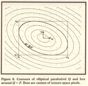
• At its core, the EWA algorithm looks at the cell-to-cell delta in source to target cell mapping, both along and across track. These deltas are used to compute the parameters for a quadratic equation defining an “ellipse of influence” from a source cell to one or more target cells.
• The “ellipse of influence” is used both to compute which target cells are affected by a source cell – a bounding box to the ellipse of influence – and to compute a weighting factor for a weighted averaging of source cells per target cell. The weighting is defined in terms of the distance of the source cell center location to the target cell center (radius of the ellipse).  Those source cells closer to the target cell are weighted more heavily than a simple linear cell-to-cell distance.

• The “ellipse of influence” provides an important technique for calculating the area of influence, in the target grid.  It is an efficient way of finding target cells when forward projecting the source data grid to the output grid. This permits a reasonably efficient “forward navigation” approach, versus more typical reverse projection algorithms.

...

• An important but not always evident aspect of the EWA algorithm is a further adjustment of the weighting factors to implement a gaussian filter to the projection processing. The gaussian filter is important to minimizing the possible effects of aliasing and moiré effects when down-sampling a larger array of source data to a smaller set of target data … data.

• Expand
  title More details...
  The topic of aliasing and moiré effects in digital image processing is complex. In brief, and perhaps unsatisfyingly so, anytime you digitize at a specific resolution, or "down-sample" from a higher resolution to lower resolution, it is possible to introduce patterns of imaging that suggest lines or curves that are not present in the original or source image. Here is one article that describes the effect, both in terms of audio sampling (where I first encountered this) and in video sampling:  https://matthews.sites.wfu.edu/misc/DigPhotog/alias/index.html.  (That is from a physics professor at Wake-Forest U., in North Carolina.  An interesting site, and not a bad explanation of what is happening). There is another article that correlates the frequency domain analysis and the various discrete filtering techniques in image processing, suggesting further that the gaussian filter used in EWA is an important if not perfect mechanism to reducing aliasing and moire patterns.  I can’t claim to fully understand this, but it does correlate the image processing world with our reprojection efforts.  Note that wherever the reprojection mapping of source data to target projection results in “downsampling” of an input area to an output area - aliasing can occur if some kind of interpolation filtering is not applied.  This is not uniform across the output dataset, as reprojection itself is not uniform, but very often applies in some area of the output: https://www.strollswithmydog.com/downsizing-algorithms-effects-on-resolution/#more-954. I’m reminded that HEG chooses a higher output resolution that minimizes downsampling effects (eliminates?), while GDAL chooses an output resolution that preserves overall grid sizing, generally at a lesser resolution, and that can introduce downsampling artifacts.  While HEG's approach may not eliminate the issue (TBD), it certainly does minimize the issue somewhat.

The algorithm itself

...